Woodbury Matrix Identity for Factor Analysis

Motivation

Given a $p$-dimensional random vector $\textbf{x}$, its generative model under factor analysis is

$\textbf{x} = \Lambda \textbf{z} + \textbf{u}$

where $\Lambda \in \mathbb{R}^{p \times k}$ is the loadings matrix and $\textbf{u} \in \mathbb{R}^{p}$ is the noise or uncertainty. The factors $\textbf{z}$ are assumed to be normal with unit variance, i.e. $\textbf{z} \sim \mathcal{N}(\textbf{0}, I_k)$. The uncertainty $\textbf{u}$ is distributed $\mathcal{N}(\textbf{0}, \Psi)$ where $\Psi$ is a diagonal matrix. This means that the random variable $\textbf{x}$ is modeled by

$\textbf{x} \sim \mathcal{N}(\textbf{0}, \underbrace{\Lambda \Lambda^{\top} + \Psi}_{\Sigma}).$

One way to view this is that since $\Lambda \Lambda^{\top}$ is a $p \times k$ matrix times a $k \times p$ matrix, it is a low-rank approximation of the covariance of $\textbf{x}$, while $\Psi$ is a correction matrix that allows $\Sigma$ to be full rank.

If you write out the log-likelihood of this model, set its derivative equal to $0$, and solve for the parameters $\Lambda$ and $\Psi$, you’ll eventually run into the fact that you need to invert $\Sigma$, i.e. this shows up in the EM updates:

$(\Lambda \Lambda^{\top} + \Psi)^{-1}$

See my previous post on factor analysis for more details. This matrix is $p \times p$, meaning that matrix inversion is $O(p^3)$ using Gauss–Jordan elimination. In Ghahramani and Hinton’s paper on a mixture of factor analyzers (Ghahramani & Hinton, 1996), they mention that $(\Lambda \Lambda^{\top} + \Psi)$ can be “efficiently inverted using the matrix inversion lemma” or the Woodbury matrix identity. This post explores what that comment means.

Woodbury matrix identity

The Woodbury matrix identity states that the inverse of a rank-$k$ correction of some matrix—in factor analysis, the full rank matrix $\Psi$ is rank-corrected by $\Lambda \Lambda^{\top}$—can be computed by doing a rank-$k$ correction to the inverse of the original matrix.

If $A$ is a $p \times p$ full rank matrix that is rank corrected by $UCV$ where $U \in \mathbb{R}^{p \times k}$, $C \in \mathbb{R}^{k \times k}$, and $V \in \mathbb{R}^{k \times p}$, then the Woodbury identity is:

$(A + UCV)^{-1} = A^{-1} - A^{-1} U (C^{-1} + V A^{-1} U)^{-1} V A^{-1}$

Wikipedia has a direct proof of this that is easy to follow. In our case, we have $A = \Psi$, $U = \Lambda$, $C = I$, and $V = \Lambda^{\top}$, giving us:

$(\Psi + \Lambda \Lambda^{\top}) = \Psi^{-1} - \Psi^{-1} \Lambda(I + \Lambda^{\top} \Psi^{-1} \Lambda)^{-1} \Lambda^{\top} \Psi^{-1}$

The critical thing to note is that

$(\overbrace{I + \Lambda^{\top} \Psi^{-1} \Lambda}^{k \times k})^{-1},$

meaning that inverting this matrix is $O(k^3)$ where we assume that $k \ll p$. Inverting $\Psi$ is easy because it is diagonal; we just replace each element in the diagonal with its reciprocal, i.e.

$\Psi^{-1}_{ii} \triangleq \frac{1}{\Psi_{ii}}$

In summary, the Woodbury matrix identity is perfect for fast matrix inversion in factor analysis. The inversion is $O(k^3)$ rather than $O(p^3)$.

Implementation

I’m starting to appreciate that while numerical linear algebra is fun—it’s the perfect combination of math, programming, and efficiency—it’s hard to get right. The Woodbury identity is a good example of what I mean.

Consider this Python function to compute the Woodbury identity given a $p$-vector $P$ that represents the diagonal elements of $\Psi$ and matrices $U$ and $V$:

import numpy as np

def woodbury(P, U, V):
    k = P.shape[1]
    # Fast inversion of diagonal Psi.
    P_inv = np.diag(1./P)
    # B is the k by k matrix to invert.
    B_inv = np.linalg.inv(np.eye(k) + V @ P_inv @ U)
    return P_inv - P_inv @ U @ B_inv @ V @ P_inv

Comparing this method to np.linalg.inv(), it is certainly faster, but it is not as fast as I would have expected (Figure $1$). What gives? In the experiments in Figure $1$, the number of samples $n$ is $100,000$, $k = 100$, and $p$, which ranges along the $x$-axis, gets as large as $10,000$. Yet NumPy is competitive with our function.

Figure 1: Comparison of `np.linalg.inv()` versus inversion using the Woodbury matrix identity. The number of samples $n$ is $100,000$ and $k = 100$. Results were computed on a standard laptop (2.3 GHz Intel Core i5, 16 GB RAM).

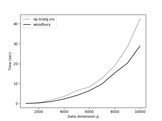
My hypothesis was that NumPy is competitive for large $p$ because woodbury() requires storing a lot of intermediate matrices and performs. To find a faster way to perform our matrix multiplications, I used einsum_path. The improved function is:

import numpy as np
    
def woodbury_einsum(P, U, V):
    k = P.shape[1]
    # Fast inversion of diagonal Psi.
    P_inv = np.diag(1./np.diag(P))
    tmp   = np.einsum('ab,bc,cd->ad',
                      V, P_inv, U,
                      optimize=['einsum_path', (1, 2), (0, 1)])
    B_inv = np.linalg.inv(np.eye(k) + tmp)
    tmp   = np.einsum('ab,bc,cd,de,ef->af',
                      P_inv, U, B_inv, V, P_inv,
                      optimize=['einsum_path', (0, 1), (0, 1), (0, 2), (0, 1)])
    return P_inv - tmp

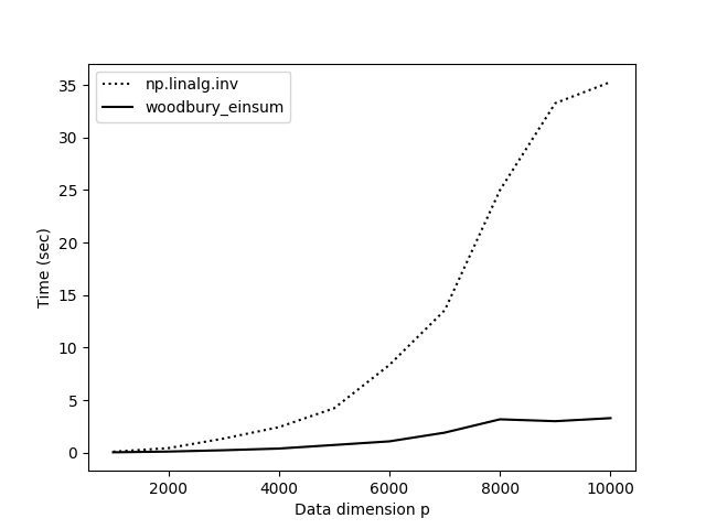
The results with woodbury_einsum() are much more satisfying (Figure $2$). Now our practical implementation starts to match our expectations based on theory.

Figure 2: Comparison of `np.linalg.inv()` versus inversion using the Woodbury matrix identity optimized with `np.einsum()`. The number of samples $n$ is $100,000$ and $k = 100$. Results were computed on a standard laptop (2.3 GHz Intel Core i5, 16 GB RAM).

But there’s an even faster way to tackle this problem. I asked how to make this function faster on StackOverflow, and someone observed that since we know P is a diagonal matrix, we can use NumPy’s broadcasting rather than explicitly performing matrix multiplications. This works because:

>>> import numpy as np
>>> A = np.array([2, 3])
>>> B = np.ones((2, 2))
>>> B * A
array([[2., 3.],
       [2., 3.]])
>>> B @ np.diag(A)
array([[2., 3.],
       [2., 3.]])

In words, when we write B * A where A is a vector, NumPy broadcasts, performing element-wise vector-vector multiplication with every row vector in B. This is mathematically equivalent to matrix multiplying B times A when A is a diagonal matrix. The code for this is (credit: Chris Swierczewski):

def woodbury_broadcasting(P, U, V):
    k = P.shape[1]
    P_inv_diag = 1./np.diag(P)
    B_inv = np.linalg.inv(np.eye(k) + (V * P_inv_diag) @ U)
    return np.diag(P_inv_diag) - (P_inv_diag.reshape(-1,1) * U @ B_inv @ V * P_inv_diag)

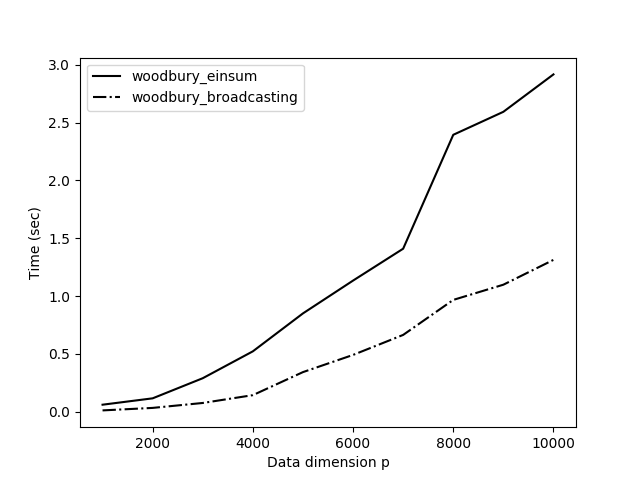
I compared this new method, woodbury_broadcasting(), to our method optimized with einsum() (Figure $3$) and the results are impressive. The new method using broadcasting is over twice as fast. This makes a lot of sense. Avoiding a couple of big matrix multiplications is obviously faster than optimizing those operations.

Figure 3: Comparison of `woodbury_einsum()` versus `woodbury_broadcasting()`. The number of samples $n$ is $100,000$ and $k = 100$. Results were computed on a standard laptop (2.3 GHz Intel Core i5, 16 GB RAM).

These kinds of problems and solutions are some of my favorite. We started with a hard problem, an algorithm that scaled cubically with the dimension of our data. But with a little math and a little programming, we were able to recover an exact solution that, for large dimensions, is several orders of magnitude faster.

Acknowledgements

I want to thank Ryan Adams for telling me to look into this identity when thinking about how to make factor analysis more scalable.