An Example of Probabilistic Machine Learning

A probabilistic approach

My first course in machine learning was Andrew Ng’s Coursera course. This class, like many other introductory resources, primarily focused on machine learning as prediction by function approximation. In this context, the goal of learning, whether we use logistic regression or neural networks, is to find parameters $\textbf{w}$ for a function $f$ such that the difference or loss $\mathcal{L}$ between the predicted values $f(\textbf{x}; \textbf{w})$ and target labels $\textbf{y}$ is minimized:

$\textbf{w}^{\star} = \arg\!\min_{\textbf{w}} \mathcal{L}(f(\textbf{x}; \textbf{w}), \textbf{y})$

But there is another way to view our data $\textbf{x}$. Rather than view our data “statically”, we can view it as random observations drawn i.i.d. from an underlying process with a true distribution $p^{\star}(\textbf{x})$. In other words, we want to find statistical parameters $\boldsymbol{\theta}$ such that:

$\textbf{x} \sim p(\textbf{x}; \boldsymbol{\theta}) \\ p(\textbf{x}; \boldsymbol{\theta}) \approx p^{\star}(\textbf{x})$

What this framing suggests is that learning is really the task of modeling this underlying process by inferring parameters $\boldsymbol{\theta}$. This inference procedure is formalized using Bayes’ theorem (I have labeled each term with its standard name in Bayesian inference):

$\overbrace{p(\boldsymbol{\theta} \mid \textbf{x})}^{\text{Posterior}} = \frac{\overbrace{p(\textbf{x} \mid \boldsymbol{\theta})}^{\text{Likelihood}} \, \overbrace{p(\boldsymbol{\theta})}^{\text{Prior}} }{\underbrace{p(\textbf{x})}_{\text{Evidence}}}$

The prior $p(\boldsymbol{\theta})$ is so-named because we specify a distribution over the parameters, thus capturing both our uncertainty and prior knowledge about the parameters. The evidence $p(\textbf{x})$ is computed by marginalizing over the parameters. This framing has many benefits, but I will focus on two: handling uncertainty and modeling generative processes.

Handling uncertainty

Without probability theory, the best function parameters $\textbf{w}^{\star}$ given our data are fixed and do not encode our uncertainty about the parameters. But with a probabilistic approach, modeling our data given this uncertainty has a natural mathematical solution, namely marginalization:

$p(\textbf{x}) = \int p(\textbf{x} \mid \boldsymbol{\theta}) p(\boldsymbol{\theta}) d \boldsymbol{\theta}$

This captures the idea that we model the data by considering all possible parameter values. Note that a central challenge for Bayesian researchers is computing this marginal distribution because it often requires either high-dimensional integration, which is computationally hard in general, or has no known analytic solution. While other researchers might focus on optimization of model parameters, Bayesian researchers often focus on techniques like MCMC and variational inference for efficiently approximating integrals.

Modeling generative processes

Every well-defined probabilistic model is also a generative model because we have learned a density. First, we sample parameters $\boldsymbol{\theta}$ from our prior and then use our learned likelihood $p(\textbf{x} \mid \boldsymbol{\theta})$ to condition on the parameters. Generating new “fantasy” data helps us to inspect what the model has learned about our observations. We’ll see a concrete example of this later.

Two clustering algorithms: $K$-means and a GMM

There’s a lot to unpack in my brief introduction, and I want to elaborate on the main points by comparing a non-probabilistic model, $K$-means, with a probabilistic model, a Gaussian mixture model. These models perform the same task of clustering, and it will be useful to compare them since only one has a probabilistic interpretation.

K-means clustering

$K$-means clustering is an unsupervised learning algorithm for partitioning $N$ data points, each with dimensionality $D$, into $K$ groups or clusters. Each cluster is represented by a single parameter $\boldsymbol{\mu}_k$, which is a $D$-vector representing the cluster’s mean. Given data $\{\textbf{x}_n \}_{n=1}^{N}$, the goal is to find cluster assignments such that the total intra-cluster squared Euclidean distance from the cluster mean is minimized. (You can also think of this as finding clusters with low variance.)

To express this as a loss, let’s introduce a one-hot vector $r_{nk}$ which denotes the cluster assignment $k$ for the $n$-th data point. Then the objective to minimize is:

$\mathcal{L} = \sum_{n=1}^{N} \sum_{k=1}^{K} r_{nk} \lVert \textbf{x}_i - \boldsymbol{\mu}_k \rVert^2_2$

Our goal is to learn the mean parameters $\{ \boldsymbol{\mu}_k \}_{k=1}^{K}$ and cluster assignments $\{r_{nk} \}_{n=1}^N$. The algorithm for fitting this model is an iterative procedure:

• Initialize the means $\boldsymbol{\mu}_k$ somehow.
• Repeat until convergence:
  • Assign each data point $\textbf{x}_i$ to its closest mean. Formally, minimize $\mathcal{L}$ w.r.t $r_{nk}$ keeping $\boldsymbol{\mu}_k$ fixed.
  • Update the means. Formally, minimize $\mathcal{L}$ w.r.t $\boldsymbol{\mu}_k$ keeping $r_{nk}$ fixed.

See Bishop, section 9.1 (Bishop, 2006) for a complete explanation and derivation. For commented code with references to Bishop, see my GitHub repository. At a high level, the algorithm is fairly straightforward and easy to visualize (see Figure 1).

Figure 1: A visualization of the $K$-means algorithm ($K=2$) on feature-scaled Old Faithful data. (a) The means are randomly initialized. (b) Each data point is assigned to one of two clusters. (c, b) Cluster means are updated based on the previous assignment step and data points are re-assigned.

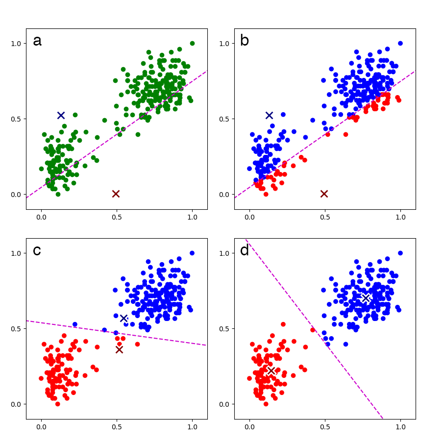
Convergence can be assessed by monitoring the loss $\mathcal{L}$ after each iteration. Once the loss has converged, we have a $K$-parameter model that allows us to cluster or label new, unseen data. For example, once the model is trained on Old Faithful data as in Figure 1, we can assign new Old Faithful data to one of the two clusters.

Gaussian mixture model

Note that nothing about $K$-means is probabilistic. There are no statistical parameters. There is no learned density. We don’t handle any uncertainty about our means $\{ \boldsymbol{\mu}_k \}_{k=1}^{K}$, and we cannot generate new data from this model.

To approach the problem from a probabilistic perspective, we could use a mixture model. A mixture model represents a density as a mixture of weighted densities. For example, a Gaussian mixture model or GMM is a mixture model in which the component densities are all Gaussian. This idea is easy to visualize with univariate Gaussians (Figure 2):

Figure 2: A Gaussian mixture model that is a weighted combination of univariate Gaussian distributions.

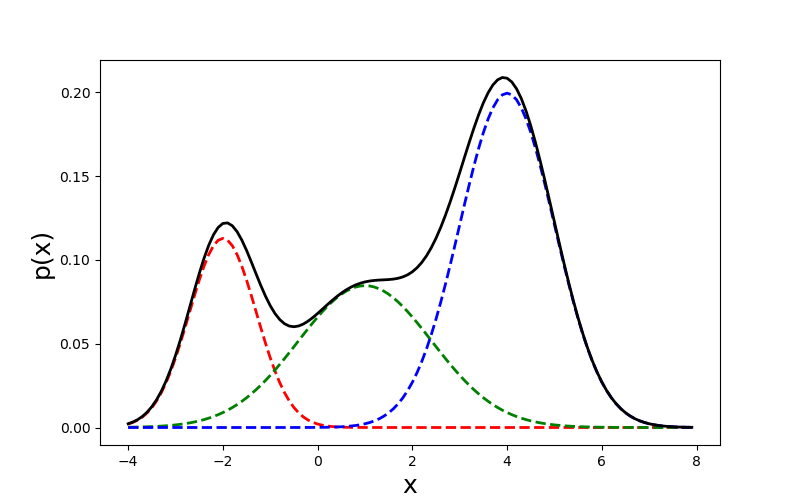
We can formalize a Gaussian mixture model as the sum of $K$ weighted Gaussian densities, called components, each with its own mean $\boldsymbol{\mu}_k$, covariance $\boldsymbol{\Sigma}_k$, and mixture weight $\pi_k$:

$p(\textbf{x}) = \sum_{k=1}^{K} \pi_k \mathcal{N}(\textbf{x} \mid \boldsymbol{\mu}_k, \boldsymbol{\Sigma}_k)$

For example, the mixture model in Figure 2 can be written as:

$p(\textbf{x}) = \color{red}{0.2 \mathcal{N}(\textbf{x} \mid -2, 0.5)} + \color{green}{0.3 \mathcal{N}(\textbf{x} \mid 1, 2)} + \color{blue}{0.5 \mathcal{N}(\textbf{x} \mid 4, 1)}$

Since $p(\textbf{x}) \geq 0$ and $\mathcal{N}(\dots) \geq 0$, this implies $\pi_k \geq 0$. Furthermore, we can see that the mixture weights must sum to $1$:

$1 = \int_x p(\textbf{x}) = \int_x \sum_{k=1}^{K} \pi_k \mathcal{N}(\textbf{x} \mid \boldsymbol{\mu}_k, \boldsymbol{\Sigma}_k) = \sum_{k=1}^{K} \pi_k \int_x \mathcal{N}(\textbf{x} \mid \boldsymbol{\mu}_k, \boldsymbol{\Sigma}_k) = \sum_{k=1}^{K} \pi_k$

Gaussian mixture models can be fit, i.e. we can learn the most likely parameters $\boldsymbol{\mu}_k$, $\boldsymbol{\Sigma}_k$, and $\pi_k$ given our data, in a variety of ways. Perhaps the most common method is expectation—maximization or the EM algorithm. At a high-level, the EM algorithm is similar to the $K$-means algorithm. It iteratively finds the most likely parameters given the data, runs until convergence, and depends on parameter initialization.

Once again, see Bishop, section 9.2 (Bishop, 2006) for an explanation and derivation, but see the Mathematics for Machine Learning by Deisenroth et al. (Deisenroth et al., 2018) for an extremely thorough derivation with proofs for the EM updates. For commented code with references to Bishop, see my GitHub repository.

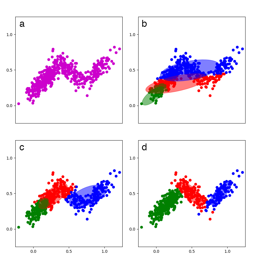
To help visualize GMMs, I created a small ($N = 500$) synthetic dataset—I am not using the Old Faithful dataset here because I want to demonstrate how GMMs handle overlapping densities—with three multivariate Gaussian densities, trained a GMM on the data, and then visualized the model at various iterations (Figure 3).

Figure 3: A visualization of fitting a Gaussian mixture model ($K=3$) on (a) synthetic data. (b) The components are randomly initialized. (c-d) The parameters of the model are iteratively updated using the EM algorithm.

Comparing the models

Now that we have a shared understanding of and notation for $K$-means and GMMs, let’s compare them. Both models are trained using iterative algorithms to find the best parameters to cluster the data. Both models use a small number of parameters to model the data; if $K$-means uses $K$ parameters, GMMs use $3 \times K$ parameters (means, variances, and weights). But a GMM is a probabilistic model, and I argued that two major benefits are (1) handling uncertainty and (2) modeling generative processes. Let’s re-consider both.

Handling uncertainty

With $K$-means, the best parameters do not capture any of our uncertainty about what the parameters should or could be. With a GMM, we handle this uncertainty by marginalization. To see this, let’s construct a GMM as a latent variable model in which each data point is generated by only one component. Using an indicator variable $z_k \in \{0, 1\}$ to indicate an assignment to the $k$-th cluster, we can write the conditional probability given $z_k$ as:

$p(\textbf{x} \mid z_k = 1) = \mathcal{N}(\textbf{x} \mid \boldsymbol{\mu}_k, \boldsymbol{\Sigma}_k)$

And if we let $\textbf{z}$ be a one hot vector of $z_k$ indicator variables, then the prior on $\textbf{z}$ and the conditional distribution are:

$p(\textbf{z}) = \prod_{k=1}^{K} (\pi_k)^{z_k} \\ p(\textbf{x} \mid \textbf{z}) = \prod_{k=1}^{K} \mathcal{N}(\textbf{x} \mid \boldsymbol{\mu}_k, \boldsymbol{\Sigma}_k)^{z_k}$

Note that if we marginalize out the latent variable, we get the same GMM model we specified earlier:

$p(\textbf{x}) = \sum_{\textbf{z}} p(\textbf{x} \mid \textbf{z}) p(\textbf{z}) = \sum_{k=1}^{K} \pi_k \mathcal{N}(\textbf{x} \mid \boldsymbol{\mu}_k, \boldsymbol{\Sigma}_k)$

This marginalization over the latent variables is the mathematical formulation of the idea that we’re considering all possible values of $\textbf{z}$.

Modeling generative processes

By sampling from a probabilistic or generative model, we can enrich our understanding of what the model learned. The latent variable construction elucidates how we sample from a GMM. Since $\textbf{z}$ depends on the mixture weights $\boldsymbol{\pi}$, we first sample cluster assignments from a categorical distribution with probabilities that are the learned mixture weights:

$\textbf{z}_{n} \sim \text{Categorical}(\boldsymbol{\pi})$

This ensures that the number of fantasy data points for each cluster is proportional to what we saw in our observed data. Next, for each sampled cluster assignment $\textbf{z}_{n}$, we sample from a multivariate Gaussian with our learned parameters $\boldsymbol{\mu}_k$ and $\boldsymbol{\Sigma}_k$:

$\textbf{x}_n \sim \mathcal{N}(\textbf{x} \mid \boldsymbol{\mu}_k, \boldsymbol{\Sigma}_k)$

I have visualized the learned density and some fantasy samples using this procedure in Figure 4.

Figure 4: (Left) The inferred GMM density given our observations in Figure 3. (Right) One hundred fantasy samples from our inferred GMM density using the sampling procedure described in the text.

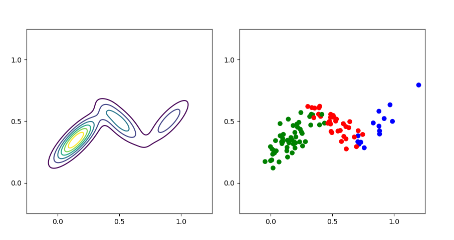
In my mind, this visualization (Figure 4) really emphasizes the mixture weights. It visualizes the mathematical fact that the blue density has the least amount of mass (Figure 4, left) and that as a consequence it is the least likely to be sampled from (Figure 4, right). We can inspect the model’s learned mixture weights and see that this is true:

$\begin{aligned} \color{green}{\text{green } \pi} \rightarrow 0.511 \\ \color{red}{\text{red } \pi} \rightarrow 0.295 \\ \color{blue}{\text{blue } \pi} \rightarrow 0.194 \end{aligned}$

The actual mixture weights for the synthetic dataset are $0.3$, $0.2$, and $0.5$ respectively.

Conclusion

There are many other benefits to probabilistic machine learning that I did not have time to mention. One that interests me greatly is compositionality through graphical models (Wainwright & Jordan, 2008). Because probabilistic models are built on probability theory, it is often much easier to understand their behavior and theoretical properties as they are combined to form larger systems. Compare this compositionality with deep neural networks. We might be able to attach two convolutional neural networks to build a multimodal system, but it is unclear how to interpret such a model, much less what its theoretical guarantees are. Probabilistic machine learning is a useful tool for composing models into complex but interpretable systems.

It took me a while to really internalize the benefits of probabilistic machine learning, and I hope I conveyed the utility of this approach by example. For additional reading from an expert on this topic, I would highly recommend Zoubin Ghahramani’s Nature review article (Ghahramani, 2015).